Do you like the article?
Share it with others —
post a link to it!

Use new possibilities of MetaTrader 5

Data label for timeseries mining (Part 2)：Make datasets with trend markers using Python

MetaTrader 5 — Expert Advisors | 18 September 2023, 13:13

1 611

Yuqiang Pan

Introduction

In the previous article, we introduced how to Label your data by observing trends on chart and save the data into a "csv" file. In this part let's think differently: start with the data itself.

We will process the data using Python. Why Python? Because it's convenient and fast, it's not means it runs fast, but Python's massive library can help us greatly reduce the development cycle.

So, let's go!

Table of contents:

Which Python library to choose

We all know that Python has a lot of excellent developers to provide a large variety of libraries, which makes it easy for us to develop, saving us a lot of development time. The following is my collection of some related python libraries, some of which are based on different architectures, some can be used for trading, some can be used for backtesting. It's including but not limited to labeled data, interested can try to study it, this article does not do a detailed introduction.

statsmodels - Python module that allows users to explore data, estimate statistical models, and perform statistical tests:http://statsmodels.sourceforge.net
dynts - Python package for timeseries analysis and manipulation:https://github.com/quantmind/dynts
PyFlux - Python library for timeseries modelling and inference (frequentist and Bayesian) on models:https://github.com/RJT1990/pyflux
tsfresh - Automatic extraction of relevant features from time series:https://github.com/blue-yonder/tsfresh
hasura/quandl-metabase - Hasura quickstart to visualize Quandl's timeseries datasets with Metabase:https://platform.hasura.io/hub/projects/anirudhm/quandl-metabase-time-series
Facebook Prophet - Tool for producing high quality forecasts for time series data that has multiple seasonality with linear or non-linear growth:https://github.com/facebook/prophet
tsmoothie - A python library for time-series smoothing and outlier detection in a vectorized way:https://github.com/cerlymarco/tsmoothie
pmdarima - A statistical library designed to fill the void in Python's time series analysis capabilities, including the equivalent of R's auto.arima function:https://github.com/alkaline-ml/pmdarima
gluon-ts - vProbabilistic time series modeling in Python:https://github.com/awslabs/gluon-ts
gs-quant - Python toolkit for quantitative finance:https://github.com/goldmansachs/gs-quant
willowtree - Robust and flexible Python implementation of the willow tree lattice for derivatives pricing:https://github.com/federicomariamassari/willowtree
financial-engineering - Applications of Monte Carlo methods to financial engineering projects, in Python:https://github.com/federicomariamassari/financial-engineering
optlib - A library for financial options pricing written in Python:https://github.com/dbrojas/optlib
tf-quant-finance - High-performance TensorFlow library for quantitative finance:https://github.com/google/tf-quant-finance
Q-Fin - A Python library for mathematical finance:https://github.com/RomanMichaelPaolucci/Q-Fin
Quantsbin - Tools for pricing and plotting of vanilla option prices, greeks and various other analysis around them:https://github.com/quantsbin/Quantsbin
finoptions - Complete python implementation of R package fOptions with partial implementation of fExoticOptions for pricing various options:https://github.com/bbcho/finoptions-dev
pypme - PME (Public Market Equivalent) calculation:https://github.com/ymyke/pypme
Blankly - Fully integrated backtesting, paper trading, and live deployment:https://github.com/Blankly-Finance/Blankly
TA-Lib - Python wrapper for TA-Lib (http://ta-lib.org/):https://github.com/mrjbq7/ta-lib
zipline - Pythonic algorithmic trading library:https://github.com/quantopian/zipline
QuantSoftware Toolkit - Python-based open source software framework designed to support portfolio construction and management:https://github.com/QuantSoftware/QuantSoftwareToolkit
finta - Common financial technical analysis indicators implemented in Pandas:https://github.com/peerchemist/finta
Tulipy - Financial Technical Analysis Indicator Library (Python bindings for tulipindicators):https://github.com/cirla/tulipy
lppls - A Python module for fitting the Log-Periodic Power Law Singularity (LPPLS) model:https://github.com/Boulder-Investment-Technologies/lppls

In there, we uses the "pytrendseries" library to process data, label trends and make datasets, because this library has the advantages of simple operation and convenient visualization. Let's start our dataset making!

Get data from MT5 client using MetaTrader5 library

Of course, the most basic thing is that python is already installed on your PC, if not, the author does not recommend installing the official version of python, but prefers to use Anaconda, which is easy to maintain. But the normal version of Anaconda is huge, integrates rich content, including visual management, editor, etc., embarrassingly I hardly use them, so I highly recommend mininconda, short and concise, simple and practical.Miniconda official website address: Miniconda :: Anaconda.org

1. Basic environment initialization

Start by creating a virtual environment and open the Anaconda Promote type：

conda create -n Data_label python=3.10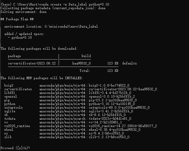

env

Enter "y" and wait for the environment to be created,then type：

conda activate Data_label

Note:When we create the conda virtual environment, remember to add python=x.xx, otherwise we will encounter inexplicable trouble during use, which is a suggestion from a person who has suffered from it!

2. Install necessary library

Install our essential library MetaTrader 5, type in the conda Promote：

pip install MetaTrader5

Install pytrendseries， type in the conda Promote：

pip install pytrendseries

3. Create python file

Open MetaEditor, find Tools->Options, fill in your python path in the python column of the Compilers option, my own path is "G:miniconda3\envs\Data_label"：

setting

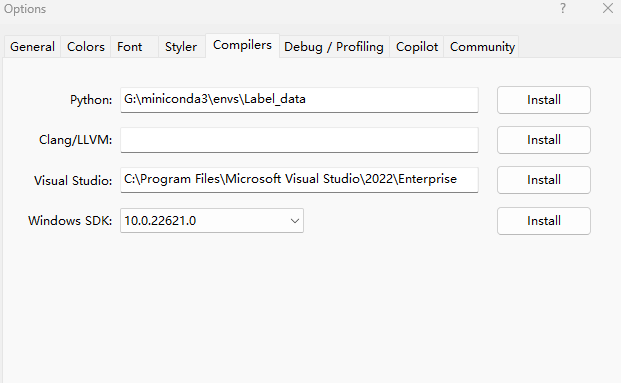
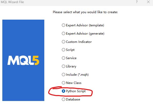
After completion, select File->New (or Ctrl + N) to create a new file, and select Python Script in the pop-up window, like this：

Click Next and type a file name，like this：

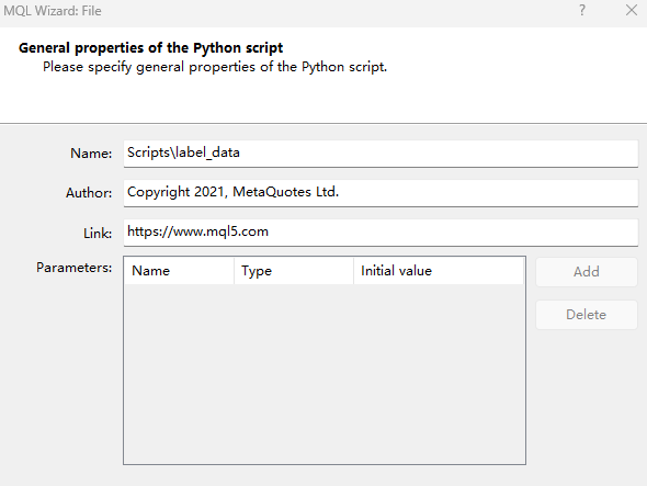
After clicking OK, the window below is shown：

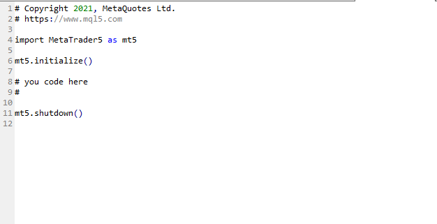
4. Connecting the client and gets data

Delete the original auto-generated code and replace it with the following code：

# Copyright 2021, MetaQuotes Ltd.
# https://www.mql5.com

import MetaTrader5 as mt

if not mt.initialize():
    print('initialize() failed!')
else:
   print(mt.version())
   mt.shutdown()

Compile and run to see if any error is reported, and if there is no problem, the following output will appear：

out

If you prompt "initialize() failed!", please add the parameter path in the initialize() function, which is the path to the client executable, as shown in the following color-weighted code：

# Copyright 2021, MetaQuotes Ltd.
# https://www.mql5.com

import MetaTrader5 as mt

if not mt.initialize("D:\\Project\\mt\\MT5\\terminal64.exe"):
    print('initialize() failed!') 
else:
    print(mt.version())
    mt.shutdown()

Everything is ready, let's get the data：

# Copyright 2021, MetaQuotes Ltd.
# https://www.mql5.com

import MetaTrader5 as mt

if not mt.initialize("D:\\Project\\mt\\MT5\\terminal64.exe"):
    print('initialize() failed!')
else:
   sb=mt.symbols_total()
   rts=None
   if sb > 0:    
     rts=mt.copy_rates_from_pos("GOLD_micro",mt.TIMEFRAME_M15,0,10000) 
   mt.shutdown()
   print(rts[0:5])

In the above code we added "sb=mt.symbols_total()" to prevent the error from being reported because no symbols were detected, and "copy_rates_from_pos("GOLD_micro", mt. TIMEFRAME_M15,0,10000)" means copying 10,000 bars from the GOLD_micro's M15 period, and the following output will be produced after compilation：

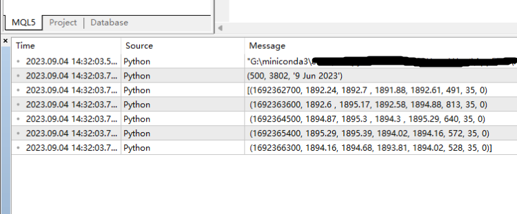
So far, we have successfully obtained the data from the client.

Data format conversion

Although we have obtained the data from the client, the data format is not we need.The data is "numpy.ndarray"，like this：

"[(1692368100, 1893.51, 1893.97,1893.08,1893.88,548, 35, 0)

(1692369000, 1893.88, 1894.51, 1893.41, 1894.51, 665, 35, 0)

(1692369900, 1894.5, 1894.91, 1893.25, 1893.62, 755, 35, 0)

(1692370800, 1893.68, 1894.7 , 1893.16, 1893.49, 1108, 35, 0)

(1692371700, 1893.5 , 1893.63, 1889.43, 1889.81, 1979, 35, 0)

(1692372600, 1889.81, 1891.23, 1888.51, 1891.04, 2100, 35, 0)

(1692373500, 1891.04, 1891.3 , 1889.75, 1890.07, 1597, 35, 0)

(1692374400, 1890.11, 1894.03, 1889.2, 1893.57, 2083, 35, 0)

(1692375300, 1893.62, 1894.94, 1892.97, 1894.25, 1692, 35, 0)

(1692376200, 1894.25, 1894.88, 1890.72, 1894.66, 2880, 35, 0)

(1692377100, 1894.67, 1896.69, 1892.47, 1893.68, 2930, 35, 0)
...
(1693822500, 1943.97, 1944.28, 1943.24, 1943.31, 883, 35, 0)

(1693823400, 1943.25, 1944.13, 1942.95, 1943.4 , 873, 35, 0)

(1693824300, 1943.4, 1944.07, 1943.31, 1943.64, 691, 35, 0)

(1693825200, 1943.73, 1943.97, 1943.73, 1943.85, 22, 35, 0)]"

So let's use pandas to convert it，the added code is marked in green:

# Copyright 2021, MetaQuotes Ltd.
# https://www.mql5.com

import MetaTrader5 as mt
import pandas as pd

if not mt.initialize("D:\\Project\\mt\\MT5\\terminal64.exe"):
    print('initialize() failed!')
else:
   print(mt.version())
   sb=mt.symbols_total()
   rts=None
   if sb > 0:
     rts=mt.copy_rates_from_pos("GOLD_micro",mt.TIMEFRAME_M15,0,1000) 
   mt.shutdown()
   rts_fm=pd.DataFrame(rts)

Now look at the data format again as below：

print(rts_fm.head(10))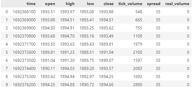

The input data must be a pandas. DataFrame format containing one column as observed data (in float or int format), so we must process the data into the format requested by pytrendseries like this:

td_data=rts_fm[['time','close']].set_index('time')

Let's see what the first 10 rows of data look like：

print(td_data.head(10))

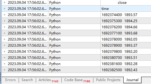
Note: The "td_data" is not our last data style, it is just a transition product for us to obtain data trends.

Now,our data is fully usable,but for the sake of subsequent operations, it is better to convert our date format to a dataframe, so we should add the following code before the "td_data=rts_fm[['time','close']].set_index('time')":

rts_fm['time']=pd.to_datetime(rts_fm['time'], unit='s')

And our output will look like this:

time	close
2023-08-18 20:45:00	1888.82000
2023-08-18 21:00:00	1887.53000
2023-08-18 21:15:00	1888.10000
2023-08-18 21:30:00	1888.98000
2023-08-18 21:45:00	1888.37000
2023-08-18 22:00:00	1887.51000
2023-08-18 22:15:00	1888.21000
2023-08-18 22:30:00	1888.73000
2023-08-18 22:45:00	1889.12000
2023-08-18 23:00:00	1889.20000

The complete code for this section：

# Copyright 2021, MetaQuotes Ltd.
# https://www.mql5.com

import MetaTrader5 as mt
import pandas as pd

if not mt.initialize("D:\\Project\\mt\\MT5\\terminal64.exe"):
    print('initialize() failed!')
else:
   print(mt.version())
   sb=mt.symbols_total()
   rts=None
   if sb > 0:
     rts=mt.copy_rates_from_pos("GOLD_micro",mt.TIMEFRAME_M15,0,1000) 
   mt.shutdown()
   rts_fm=pd.DataFrame(rts)
   rts_fm['time']=pd.to_datetime(rts_fm['time'], unit='s')
   td_data=rts_fm[['time','close']].set_index('time')
   print(td_data.head(10))

Label data

1. Get trend data

First import the "pytrendseries" package：

import pytrendseries as pts

We use the "pts.detecttrend()" function to find trend, then define "td" variable for this function and there are two options for this parameter-"downtrend" or "uptrend"：

td='downtrend' # or "uptrend"

We need another parameter "wd" as maximum period of a trend:

wd=120

There is also a parameter that may or may not be defined, but I personally think it is better to define it，this parameter specifies the minimum period of the trend：

limit=6

Now we can fill the parameters into the function to get the trend：

trends=pts.detecttrend(td_data,trend=td,limit=limit,window=wd)

Then check the result：

print(trends.head(15))

	from	to	price0	price1	index_from	index_to	time_span	drawdown
1	2023-08-21 01:00:00	2023-08-21 02:15:00	1890.36000	1889.24000	13	18	5	0.00059
2	2023-08-21 03:15:00	2023-08-21 04:45:00	1890.61000	1885.28000	22	28	6	0.00282
3	2023-08-21 08:00:00	2023-08-21 13:15:00	1893.30000	1886.86000	41	62	21	0.00340
4	2023-08-21 15:45:00	2023-08-21 17:30:00	1896.99000	1886.16000	72	79	7	0.00571
5	2023-08-21 20:30:00	2023-08-21 22:30:00	1894.77000	1894.12000	91	99	8	0.00034
6	2023-08-22 04:15:00	2023-08-22 05:45:00	1896.19000	1894.31000	118	124	6	0.00099
7	2023-08-22 06:15:00	2023-08-22 07:45:00	1896.59000	1893.80000	126	132	6	0.00147
8	2023-08-22 13:00:00	2023-08-22 16:45:00	1903.38000	1890.17000	153	168	15	0.00694
9	2023-08-22 19:00:00	2023-08-22 21:15:00	1898.08000	1896.25000	177	186	9	0.00096
10	2023-08-23 04:45:00	2023-08-23 06:00:00	1901.46000	1900.25000	212	217	5	0.00064
11	2023-08-23 11:30:00	2023-08-23 13:30:00	1904.84000	1901.42000	239	247	8	0.00180
12	2023-08-23 19:45:00	2023-08-23 23:30:00	1919.61000	1915.05000	272	287	15	0.00238
13	2023-08-24 09:30:00	2023-08-25 09:45:00	1921.91000	1912.93000	323	416	93	0.00467
14	2023-08-25 15:00:00	2023-08-25 16:30:00	1919.88000	1913.30000	437	443	6	0.00343
15	2023-08-28 04:15:00	2023-08-28 07:15:00	1916.92000	1915.07000	486	498	12	0.00097

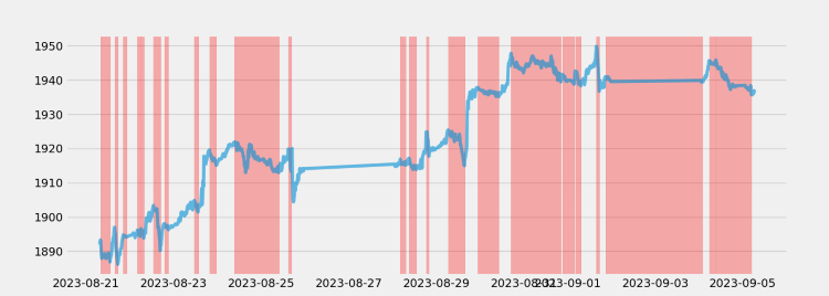
You can also visualize the result through the function "pts.vizplot.plot_trend()":

pts.vizplot.plot_trend(td_data,trends)

Similarly, we can look at the uptrend by code：

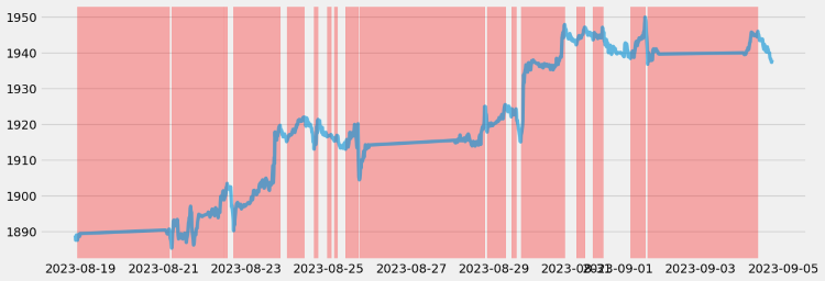
td="uptrend"
wd=120
limit=6

trends=pts.detecttrend(td_data,trend=td,limit=limit,window=wd)
print(trends.head(15))
pts.vizplot.plot_trend(td_data,trends)

The result is this：

	from	to	price0	price1	index_from	index_to	time_span	drawup
1	2023-08-18 22:00:00	2023-08-21 03:15:00	1887.51000	1890.61000	5	22	17	0.00164
2	2023-08-21 04:45:00	2023-08-22 10:45:00	1885.28000	1901.35000	28	144	116	0.00852
3	2023-08-22 11:15:00	2023-08-22 13:00:00	1898.78000	1903.38000	146	153	7	0.00242
4	2023-08-22 16:45:00	2023-08-23 19:45:00	1890.17000	1919.61000	168	272	104	0.01558
5	2023-08-23 23:30:00	2023-08-24 09:30:00	1915.05000	1921.91000	287	323	36	0.00358
6	2023-08-24 15:30:00	2023-08-24 17:45:00	1912.97000	1921.24000	347	356	9	0.00432
7	2023-08-24 23:00:00	2023-08-25 01:15:00	1916.41000	1917.03000	377	382	5	0.00032
8	2023-08-25 03:15:00	2023-08-25 04:45:00	1915.20000	1916.82000	390	396	6	0.00085
9	2023-08-25 09:45:00	2023-08-25 17:00:00	1912.93000	1920.03000	416	445	29	0.00371
10	2023-08-25 17:45:00	2023-08-28 18:30:00	1904.37000	1924.86000	448	543	95	0.01076
11	2023-08-28 20:00:00	2023-08-29 06:30:00	1917.74000	1925.41000	549	587	38	0.00400
12	2023-08-29 10:00:00	2023-08-29 12:45:00	1922.00000	1924.21000	601	612	11	0.00115
13	2023-08-29 15:30:00	2023-08-30 17:00:00	1914.98000	1947.79000	623	721	98	0.01713
14	2023-08-30 23:45:00	2023-08-31 04:45:00	1942.09000	1947.03000	748	764	16	0.00254
15	2023-08-31 09:30:00	2023-08-31 15:00:00	1943.52000	1947.00000	783	805	22	0.00179

2. Label the data

1). Parse the data format

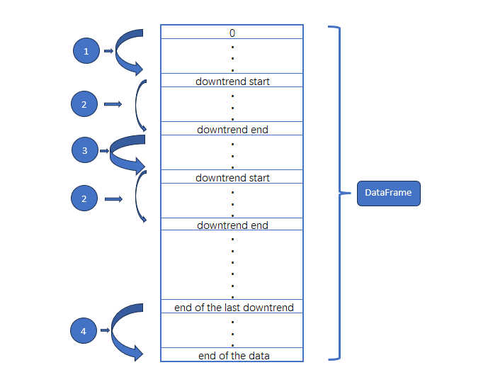
① means the beginning of the data to the beginning of the first downtrend，let's assume this is an uptrend;

② means the downtrend；

③ means the uptrend in the middle of the data;

④ means the end of last downtrend.

So we must implement the label logic for these four parts.

2). label logic

Let's start by defining some basic variables：

rts_fm['trend']=0
rts_fm['trend_index']=0
max_len_rts=len(rts_fm)
max_len=len(trends)
last_start=0
last_end=0

Traverse the "trends" variable with a for loop to get the beginning and end of each piece of data:

for trend in trends.iterrows():
        pass

Gets the start and end indexes for each segment：

for trend in trends.iterrows():
    start=trend[1]['index_from']
    end=trend[1]['index_to']

Because the rts_fm["trend"] itself has been initialized to 0, there is no need to change the "trend" column of the uptrend, but we need to see if the start of the data is a downtrend，if it is not a downtrend, we assumed it to be an uptrend：

for trend in trends.iterrows():
    start=trend[1]['index_from']
    end=trend[1]['index_to']

    if trend[0]==1 and start!=0:
        # Since the rts_fm["trend"] itself has been initialized to 0, there is no need to change the "trend" column
        rts_fm['trend_index'][0:start]=list(range(0,start))

As the same as the beginning of the data, we need to see if it ends in a downtrend at the end of the data:

for trend in trends.iterrows():
    start=trend[1]['index_from']
    end=trend[1]['index_to']

    if trend[0]==1 and start!=0:
        # Since the rts_fm["trend"] itself has been initialized to 0, there is no need to change the "trend" column
        rts_fm['trend_index'][0:start]=list(range(0,start))
    elif trend[0]==max_len and end!=max_len_rts-1:
	#we need to see if it ends in a downtrend at the end of the data
        rts_fm['trend_index'][last_end+1:len(rts_fm)]=list(range(0,max_len_rts-last_end-1))

Process the uptrend segments other than the beginning and end of the data：

for trend in trends.iterrows():
    start=trend[1]['index_from']
    end=trend[1]['index_to']

    if trend[0]==1 and start!=0:
        # Since the rts_fm["trend"] itself has been initialized to 0, there is no need to change the "trend" column
        rts_fm['trend_index'][0:start]=list(range(0,start))
    elif trend[0]==max_len and end!=max_len_rts-1:
        #we need to see if it ends in a downtrend at the end of the data
        rts_fm['trend_index'][last_end+1:len(rts_fm)]=list(range(0,max_len_rts-last_end-1))
    else:
        #Process the uptrend segments other than the beginning and end of the data
        rts_fm["trend_index"][last_end+1:start]=list(range(0,start-last_end-1))

Process each segments of the downtrend：

for trend in trends.iterrows():
    start=trend[1]['index_from']
    end=trend[1]['index_to']

    if trend[0]==1 and start!=0:
        # Since the rts_fm["trend"] itself has been initialized to 0, there is no need to change the "trend" column
        rts_fm['trend_index'][0:start]=list(range(0,start))
    elif trend[0]==max_len and end!=max_len_rts-1:
        #we need to see if it ends in a downtrend at the end of the data
        rts_fm['trend_index'][last_end+1:len(rts_fm)]=list(range(0,max_len_rts-last_end-1))
    else:
        #Process the uptrend segments other than the beginning and end of the data
        rts_fm["trend_index"][last_end+1:start]=list(range(0,start-last_end-1))
    
    #Process each segments of the downtrend
    rts_fm["trend"][start:end+1]=1
    rts_fm["trend_index"][start:end+1]=list(range(0,end-start+1))
    last_start=start
    last_end=end

3). supplement
We assume that the beginning and end of the data are uptrending, and if you think this is not precise enough, you can also remove the beginning and ending parts. To do this, add the following code after the for loop ends:

rts_fm['trend']=0
rts_fm['trend_index']=0
max_len_rts=len(rts_fm)
max_len=len(trends)
last_start=0
last_end=0
for trend in trends.iterrows():
    start=trend[1]['index_from']
    end=trend[1]['index_to']

    if trend[0]==1 and start!=0:
        # Since the rts_fm["trend"] itself has been initialized to 0, there is no need to change the "trend" column
        rts_fm['trend_index'][0:start]=list(range(0,start))
    elif trend[0]==max_len and end!=max_len_rts-1:
        #we need to see if it ends in a downtrend at the end of the data
        rts_fm['trend_index'][last_end+1:len(rts_fm)]=list(range(0,max_len_rts-last_end-1))
    else:
        #Process the uptrend segments other than the beginning and end of the data
        rts_fm["trend_index"][last_end+1:start]=list(range(0,start-last_end-1))
    
    #Process each segments of the downtrend
    rts_fm["trend"][start:end+1]=1
    rts_fm["trend_index"][start:end+1]=list(range(0,end-start+1))
    last_start=start
    last_end=end
rts_fm=rts_fm.iloc[trends.iloc[0,:]['index_from']:end,:]

3.Check

Once we've done that, let's see if our data meets our expectations(The example looks only at the first 25 pieces of data)：

rts_fm.head(25)

	time	open	high	low	close	tick_volume	spread	trend	trend_index
0	2023-08-22 11:30:00	1898.80000	1899.72000	1898.22000	1899.30000	877	35	0	0
1	2023-08-22 11:45:00	1899.31000	1899.96000	1898.84000	1899.81000	757	35	0	1
2	2023-08-22 12:00:00	1899.86000	1900.50000	1899.24000	1900.01000	814	35	0	2
3	2023-08-22 12:15:00	1900.05000	1901.26000	1899.99000	1900.48000	952	35	0	3
4	2023-08-22 12:30:00	1900.48000	1902.44000	1900.17000	1902.19000	934	35	0	4
5	2023-08-22 12:45:00	1902.23000	1903.59000	1902.21000	1902.64000	891	35	0	5
6	2023-08-22 13:00:00	1902.69000	1903.94000	1902.24000	1903.38000	873	35	1	0
7	2023-08-22 13:15:00	1903.40000	1904.29000	1901.71000	1902.08000	949	35	1	1
8	2023-08-22 13:30:00	1902.10000	1903.37000	1902.08000	1902.63000	803	35	1	2
9	2023-08-22 13:45:00	1902.64000	1902.75000	1901.75000	1901.80000	1010	35	1	3
10	2023-08-22 14:00:00	1901.79000	1902.47000	1901.33000	1901.96000	800	35	1	4
11	2023-08-22 14:15:00	1901.94000	1903.04000	1901.72000	1901.73000	785	35	1	5
12	2023-08-22 14:30:00	1901.71000	1902.62000	1901.66000	1902.38000	902	35	1	6
13	2023-08-22 14:45:00	1902.38000	1903.23000	1901.96000	1901.96000	891	35	1	7
14	2023-08-22 15:00:00	1901.94000	1903.25000	1901.64000	1902.41000	1209	35	1	8
15	2023-08-22 15:15:00	1902.39000	1903.00000	1898.97000	1899.87000	1971	35	1	9
16	2023-08-22 15:30:00	1899.86000	1901.17000	1896.72000	1896.85000	2413	35	1	10
17	2023-08-22 15:45:00	1896.85000	1898.15000	1896.12000	1897.26000	2010	35	1	11
18	2023-08-22 16:00:00	1897.29000	1897.45000	1895.52000	1895.97000	2384	35	1	12
19	2023-08-22 16:15:00	1895.96000	1896.31000	1893.87000	1894.48000	1990	35	1	13
20	2023-08-22 16:30:00	1894.43000	1894.60000	1892.64000	1893.38000	2950	35	1	14
21	2023-08-22 16:45:00	1893.48000	1894.17000	1888.94000	1890.17000	2970	35	1	15
22	2023-08-22 17:00:00	1890.19000	1894.53000	1889.94000	1894.20000	2721	35	0	0
23	2023-08-22 17:15:00	1894.18000	1894.73000	1891.51000	1891.71000	1944	35	0	1
24	2023-08-22 17:30:00	1891.74000	1893.70000	1890.91000	1893.59000	2215	35	0	2

You can see that we successfully added trend types and trend index markers to the data.

4. Save the file

We can save the data in most file formats that we want，you can save as a JSON file using the to_json() method, you can save as an HTML file using the to_html() method, and so on.Only saving as a CSV file is used here as a demonstration，at the end of the code to add：

rts_fm.to_csv('GOLD_micro_M15.csv')

Manual proofreading

At this point, we have done the basic work，but if we want to get more precise data, we need further human intervention, we will only point out a few directions here, and will not make a detailed demonstration.

1.Data integrity checks

Completeness refers to whether data information is missing, which may be the absence of the entire data or the absence of a field in the data. Data integrity is one of the most fundamental evaluation criteria for data quality.For example，if the previous data in the M15 period stock market data differs by 2 hours from the next data, then we need to use the corresponding tools to complete the data.Of course, it is generally difficult to get foreign exchange data or stock market data obtained from our client terminal, but if you get time series from other sources such as traffic data or weather data , you need to pay special attention to this situation.

The integrity of data quality is relatively easy to assess, and can generally be evaluated by the recorded and unique values in the data statistics. For example, if a stock price data in the previous period the Close price is 1000, but the Open price becomes 10 in the next period, you need to check if the data is missing.

2.Check the accuracy of data labeling

From the perspective of this article, the data labeling method we implemented above may have certain vulnerabilities, we can not only rely on the methods provided in the pytrendseries library to obtain accurate labeling data, but also need to visualize the data, observe whether the trend classification of the data is too susceptible or dullness, so that some key information is missed, at this time we need to analyze the data, if should be broken down then broken down , if should be merged needs to be merged.This work requires a lot of effort and time to complete, and concrete examples are not provided here for the time being.

Accuracy refers to whether the information recorded in the data and whether the data is accurate, and whether the information recorded in the data is abnormal or wrong. Unlike consistency, data with accuracy issues is not just inconsistencies in rules. Consistency issues can be caused by inconsistent rules for data logging, but not necessarily errors.

3.Do some basic statistical verification to see if the labels are reasonable

Integrity Distribution:Quickly and intuitively see the completeness of the data set.
Heatmap:Heat maps make it easy to observe the correlation between two variables.
Hierarchical Clustering:You can see whether the different classes of your data are closely related or scattered.

Of course, it's not just about the above methods.

Summary

Reference: GitHub - rafa-rod/pytrendseries

The complete code is shown below：

# Copyright 2021, MetaQuotes Ltd.
# https://www.mql5.com

import MetaTrader5 as mt
import pandas as pd
import pytrendseries as pts

if not mt.initialize("D:\\Project\\mt\\MT5\\terminal64.exe"):
    print('initialize() failed!')
else:
   print(mt.version())
   sb=mt.symbols_total()
   rts=None
   if sb > 0:
     rts=mt.copy_rates_from_pos("GOLD_micro",mt.TIMEFRAME_M15,0,1000) 
   mt.shutdown()
   rts_fm=pd.DataFrame(rts)
   rts_fm['time']=pd.to_datetime(rts_fm['time'], unit='s')
   td_data=rts_fm[['time','close']].set_index('time')
   # print(td_data.head(10))

td='downtrend' # or "uptrend"
wd=120
limit=6

trends=pts.detecttrend(td_data,trend=td,limit=limit,window=wd)
# print(trends.head(15))
# pts.vizplot.plot_trend(td_data,trends)

rts_fm['trend']=0
rts_fm['trend_index']=0
max_len_rts=len(rts_fm)
max_len=len(trends)
last_start=0
last_end=0
for trend in trends.iterrows():
    start=trend[1]['index_from']
    end=trend[1]['index_to']

    if trend[0]==1 and start!=0:
        # Since the rts_fm["trend"] itself has been initialized to 0, there is no need to change the "trend" column
        rts_fm['trend_index'][0:start]=list(range(0,start))
    elif trend[0]==max_len and end!=max_len_rts-1:
        #we need to see if it ends in a downtrend at the end of the data
        rts_fm['trend_index'][last_end+1:len(rts_fm)]=list(range(0,max_len_rts-last_end-1))
    else:
        #Process the uptrend segments other than the beginning and end of the data
        rts_fm["trend_index"][last_end+1:start]=list(range(0,start-last_end-1))
    
    #Process each segments of the downtrend
    rts_fm["trend"][start:end+1]=1
    rts_fm["trend_index"][start:end+1]=list(range(0,end-start+1))
    last_start=start
    last_end=end
#rts_fm=rts_fm.iloc[trends.iloc[0,:]['index_from']:end,:]
rts_fm.to_csv('GOLD_micro_M15.csv')

Note:

1.Remember that if you add path in the mt.initialize() function like this: mt.initialize("D:\\Project\\mt\\MT5\\terminal64.exe"), be sure to replace it with the location of your own client executable, not mine.

2.If you can't find the 'GOLD_micro_M15.csv' file, look for it in the client root, e.g. my file is in the path:"D:\\Project\\mt\\MT5\\".

Thank you for your patience in reading, I hope you gain something and wish you a happy life, and see you in the next chapter!

Attached files |

Download ZIP

Label_data.py (1.84 KB)

Warning: All rights to these materials are reserved by MetaQuotes Ltd. Copying or reprinting of these materials in whole or in part is prohibited.

Similar articles